Last Update: March 6, 2020
Algorithm learning consists of algorithm training within training data subset for optimal parameters estimation and algorithm testing within testing data subset using previously optimized parameters. This corresponds to a supervised regression machine learning task.
This topic is part of Machine Trading Analysis with R course. Feel free to take a look at Course Curriculum.
This tutorial has an educational and informational purpose and doesn’t constitute any type of trading or investment advice. All content, including code and data, is presented for personal educational use exclusively and with no guarantee of exactness of completeness. Past performance doesn’t guarantee future results. Please read full Disclaimer.
An example of supervised boundary-based machine learning algorithm is support vector machine [1] which consists of predicting output target feature by separating output target and input predictor features data into optimal hyper-planes. Output target prediction error regularization and time series cross-validation are used for lowering variance error source generated by a greater model complexity.
1. Kernel function.
Kernel function consists of transforming output target and input predictors feature data into higher dimensional feature space to perform linear separation into optimal hyper-planes. For supervised machine learning, linear, polynomial, Gaussian radial basis or hyperbolic tangent sigmoid functions are used.
1.1. Kernel function formula notation.
Where = linear kernel function,
= input predictor features data,
= output target feature data.
2. Algorithm definition.
Quadratic programming consists of finding optimal width coefficients by maximizing separation between output target and input predictors features data support vectors subject to output target prediction errors regularization and tolerance margin.
2.1. Algorithm formula notation.
Where = support vectors margin width coefficient,
= output target feature prediction error regularization coefficient,
= output target feature prediction error or distance outside of margins,
= output target feature data,
= input predictor features data
= intercept coefficient or bias,
= output target feature prediction error tolerance margin,
= number of observations.
3. R script code example.
3.1. Load R packages [2].
library('quantmod')
library('e1071')
3.2. Support vector machine regression data reading, target and predictor features creation, training and testing ranges delimiting.
- Data: S&P 500® index replicating ETF (ticker symbol: SPY) daily adjusted close prices (2007-2015).
- Data daily arithmetic returns used for target feature (current day) and predictor feature (previous day).
- Target and predictor features creation, training and testing ranges delimiting not fixed and only included for educational purposes.
data <- read.csv("Support-Vector-Machine-Regression-Data.txt",header=T)
spy <- xts(data[,2],order.by=as.Date(data[,1]))
rspy <- dailyReturn(spy)
rspy1 <- lag(rspy,k=1)
rspyall <- cbind(rspy,rspy1)
colnames(rspyall) <- c('rspy','rspy1')
rspyall <- na.exclude(rspyall)rspyt <- window(rspyall,end='2014-01-01')
rspyf <- window(rspyall,start='2014-01-01')3.3. Support vector machine regression fitting, output and chart.
- Support vector machine fitting within training range.
- Support vector machine fitting kernel function, cost regularization coefficient and epsilon tolerance margin not fixed and only included for educational purposes.
svmt <- svm(rspy~rspy1,data=rspyt,kernel='linear',cost=1.0,epsilon=0.1)
svmtfv <- predict(svmt,data=rspyt$rspy1)
In:
coef(svmt)Out:
(Intercept) rspy1
0.04709576 -0.05851165plot(y=coredata(rspyt$rspy),x=coredata(rspyt$rspy1))
points(y=svmtfv,x=coredata(rspyt$rspy1),col='blue')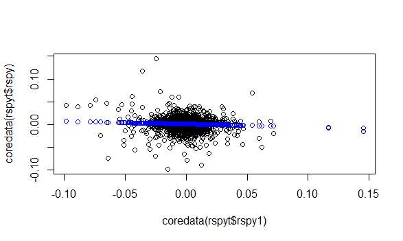
4. References.
[1] Harris Drucker, Christopher Burges, Linda Kaufman, Alexander Smola and Vladimir Vapnik. “Support Vector Regression Machines”. MIT Press. 1997.
[2] Jeffrey A. Ryan and Joshua M. Ulrich. “quantmod: Quantitative Financial Modelling Framework”. R package version 0.4-15. 2019.
David Meyer, Evgenia Dimitriadou, Kurt Hornik, Andreas Weingessel and Friedrich Leisch. “e1071: Misc Functions of the Department of Statistics, Probability Theory Group (Formerly: E1071), TU Wien”. R package version 1.7-3. 2019.