Last Update: February 6, 2020
Pairs identification consists of searching for paired asset prices which moved together based on fundamental or technical factors and initially tested through their returns’ correlation coefficient.
This topic is part of Pairs Trading Analysis with R course. Feel free to take a look at Course Curriculum.
This tutorial has an educational and informational purpose and doesn’t constitute any type of trading or investment advice. All content, including code and data, is presented for personal educational use exclusively and with no guarantee of exactness of completeness. Past performance doesn’t guarantee future results. Please read full Disclaimer.
Initial pairs identification is done through correlation coefficient which consists of measuring the degree to which paired assets prices returns moved together taking into consideration their standard deviation. It is used for evaluating short-term relationships.
1. Formula notation.
Where = paired assets
and
prices arithmetic returns’ correlation coefficient,
= current period asset
prices arithmetic return,
= current period asset
prices arithmetic return,
= asset
prices arithmetic returns arithmetic mean and
= asset
prices arithmetic returns arithmetic mean.
2. R script code example.
2.1. Load R package [1].
library('quantmod')2.2. Paired prices returns’ correlation data reading, training and testing ranges delimiting.
- Data: MSCI® Germany and France indexes replicating ETFs (ticker symbols: EWG and EWQ) daily adjusted close prices (2007-2016).
- Training and testing ranges delimiting not fixed and only included for educational purposes.
data <- read.csv('Paired-Prices-Returns-Correlation-Data.txt',header=T)
data <- xts(data[,2:3],order.by=as.Date(data[,1]))
tdata <- data['::2014-12-31']
fdata <- data['2015-01-02::']2.3. Paired prices chart.
- Paired prices chart within training range.
tger <- tdata[,1]
tfra <- tdata[,2]
plot(as.zoo(tger),main='Paired Prices Chart',xlab='',ylab='')
par(new=T)
plot(as.zoo(tfra),col='blue',xaxt='n',yaxt='n',xlab='',ylab='')
axis(side=4)
legend('bottomright',col=c('black','blue'),lty=1,legend=c('tger','tfra'),cex=0.8)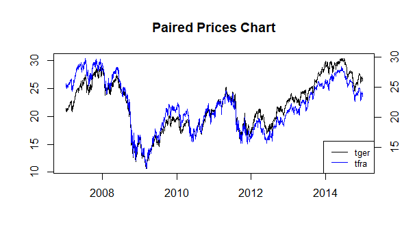
2.4. Paired prices returns’ correlation calculation.
- Paired prices returns’ correlation calculation within training range.
rtger <- dailyReturn(tger)
rtfra <- dailyReturn(tfra)
colnames(rtger) <- 'rtger'
colnames(rtfra) <- 'rtfra'
In:
cor(rtger,rtfra)Out:
rtfra
rtger 0.95144043. References.
[1] Jeffrey A. Ryan and Joshua M. Ulrich. “quantmod: Quantitative Financial Modelling Framework”. R package version 0.4-15. 2019.