Multicollinearity Test with R

Last Update: March 2, 2020

Multiple regression assumptions consist of independent variables correct specification, independent variables no linear dependence, regression correct functional form, residuals no autocorrelation, residuals homoscedasticity and residuals normality.

This topic is part of Multiple Regression Analysis with R course. Feel free to take a look at Course Curriculum.

This tutorial has an educational and informational purpose and doesn’t constitute any type of business, forecasting, trading or investment advice. All content, including code and data, is presented for personal educational use exclusively and with no guarantee of exactness of completeness. Past performance doesn’t guarantee future results. Please read full Disclaimer.

No linear dependence or no multicollinearity consists of regression independent variables not being highly correlated.

This is evaluated through multicollinearity test which consists of calculating an inverted correlation matrix of independent variables and assessing its main diagonal values.

• If main diagonal values were greater than five but less than ten, independent variables might have been highly correlated.
• If main diagonal values were greater than ten, independent variables were highly correlated.

1. R script code example.

1.1. Load R packages [1].

library('quantmod')
library('MASS')
library('corrplot')

1.2. Multicollinearity test data.

• Data: S&P 500® index replicating ETF (ticker symbol: SPY) adjusted close prices arithmetic monthly returns, 1 Year U.S. Treasury Bill Yield, 10 Years U.S. Treasury Note Yield, Merrill Lynch U.S. High Yield Corporate Bond Index Yield effective monthly yields, U.S. Consumer Price Index, U.S. Producer Price Index monthly inflations or deflations, West Texas Intermediate Oil prices arithmetic monthly returns, U.S. Industrial Production Index value, U.S. Personal Consumption Expenditures arithmetic monthly changes (1997-2016).

data <- read.csv('Multicollinearity-Test-Data.txt',header=T)
data <- xts(data[,2:10],order.by=as.Date(data[,1]))

1. 3. Multicollinearity test calculation and chart.

• Multicollinearity test done only on independent variables.

ivar <- data[,2:9]
ivarcor <- cor(ivar) 
ivaricor <- ginv(ivarcor)
colnames(ivaricor) <- colnames(ivar)
rownames(ivaricor) <- colnames(ivar)

In:
ivaricor

Out:
               t1y        t10y     hyield         cpi         ppi
t1y     5.46793530 -5.27291477  0.7765024 -0.27503564  0.57042222
t10y   -5.27291477  6.61777724 -1.6307083 -0.01601086 -0.58422061
hyield  0.77650240 -1.63070830  1.7978549  0.15668013  0.30072957
cpi    -0.27503564 -0.01601086  0.1566801  2.70827367 -1.84852043
ppi     0.57042222 -0.58422061  0.3007296 -1.84852043  3.07937188
oil    -0.02487049  0.13332779 -0.1608662 -0.14447297 -0.92231773
indpro  0.35682332 -0.79214915  0.6493560  0.26548724 -0.11232369
pce    -0.02339095 -0.27744782  0.2850202 -0.39687520  0.08226906
               oil     indpro         pce
t1y    -0.02487049  0.3568233 -0.02339095
t10y    0.13332779 -0.7921491 -0.27744782
hyield -0.16086624  0.6493560  0.28502023
cpi    -0.14447297  0.2654872 -0.39687520
ppi    -0.92231773 -0.1123237  0.08226906
oil     1.68617333 -0.0339357 -0.18419807
indpro -0.03393570  1.3533350 -0.19565742
pce    -0.18419807 -0.1956574  1.36553413

corrplot(ivaricor,method='number',is.corr=F)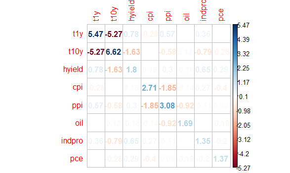

2. References.

[1] Jeffrey A. Ryan and Joshua M. Ulrich. “quantmod: Quantitative Financial Modelling Framework”. R package version 0.4-15. 2019.

W. N. Venables and B. D. Ripley. “Modern Applied Statistics with S”. Fourth Edition. Springer. 2002.

Taiyun Wei and Viliam Simko. “corrplot”: Visualization of a Correlation Matrix. R package version 0.84. 2017.