Last Update: February 6, 2020
Supervised machine learning consists of finding which class output target data belongs to or predicting its value by mapping its optimal relationship with input predictors data. Main supervised learning tasks are classification and regression.
This topic is part of Regression Machine Learning with R course. Feel free to take a look at Course Curriculum.
This tutorial has an educational and informational purpose and doesn’t constitute any type of forecasting, business, trading or investment advice. All content, including code and data, is presented for personal educational use exclusively and with no guarantee of exactness of completeness. Past performance doesn’t guarantee future results. Please read full Disclaimer.
An example of supervised learning algorithm is decision tree regression [1] which consists of predicting output target feature by optimally recursive binary node splitting of output target and input predictor features data into incrementally smaller nodes. Top node is root node, internal nodes are decision nodes and terminal nodes are leaf nodes. Tree pruning and time series cross-validation are used for lowering variance error source generated by a greater model complexity.
1. Algorithm definition.
Classification and regression trees (CART) algorithm consists of greedy top-down approach for finding optimal recursive binary node splits by locally minimizing variance at terminal nodes measured through sum of squared errors function at each stage.
2. Formula notation.
Where = output target feature data,
= terminal node output target feature mean,
= number of observations,
= number of observations in terminal node.
3. R script code example.
3.1. Load R packages [2].
library('quantmod')
library('tree')
3.2. Decision tree regression data reading, target and predictor features creation, training and testing ranges delimiting.
- Data: S&P 500® index replicating ETF (ticker symbol: SPY) daily adjusted close prices (2007-2015).
- Data daily arithmetic returns used for target feature (current day) and predictor feature (previous day).
- Target and predictor features creation, training and testing ranges delimiting not fixed and only included for educational purposes.
data <- read.csv("Decision-Tree-Regression-Data.txt",header=T)
spy <- xts(data[,2],order.by=as.Date(data[,1]))
rspy <- dailyReturn(spy)
rspy1 <- lag(rspy,k=1)
rspyall <- cbind(rspy,rspy1)
colnames(rspyall) <- c('rspy','rspy1')
rspyall <- na.exclude(rspyall)rspyt <- window(rspyall,end='2014-01-01')
rspyf <- window(rspyall,start='2014-01-01')3.3. Decision tree regression fitting, output and chart.
- Decision tree fitting within training range.
In:
dtt <- tree(rspy~rspy1,data=rspyt)
dtt$frame
Out:
var n dev yval splits.cutleft splits.cutright
1 rspy1 1761 0.380468660 0.0003432465 <-0.0646011 >-0.0646011
2 <leaf> 6 0.004074513 0.0329532693
3 <leaf> 1755 0.369991852 0.0002317593plot(dtt)
text(dtt)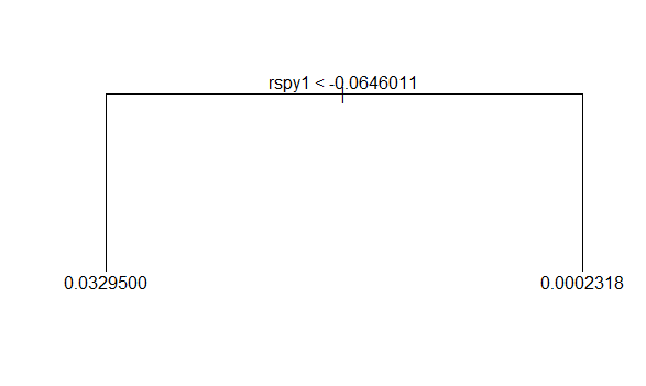
4. References.
[1] Breiman L, Friedman JH, Olshen RA, Stone CJ. “Classification and Regression Trees”. CRC Press. 1984.
[2] Jeffrey A. Ryan and Joshua M. Ulrich. “quantmod: Quantitative Financial Modelling Framework”. R package version 0.4-15. 2019.
Brian Ripley. “tree: Classification and Regression Trees”. R package version 1.0-40. 2019.