Last Update: February 10, 2020
Supervised deep learning consists of using multi-layered algorithms for finding which class output target data belongs to or predicting its value by mapping its optimal relationship with input predictors data. Main supervised deep learning tasks are classification and regression.
This topic is part of Deep Learning Regression with R course. Feel free to take a look at Course Curriculum.
This tutorial has an educational and informational purpose and doesn’t constitute any type of forecasting, business, trading or investment advice. All content, including code and data, is presented for personal educational use exclusively and with no guarantee of exactness of completeness. Past performance doesn’t guarantee future results. Please read full Disclaimer.
An example of supervised deep learning algorithm is artificial neural network [1] which consists of predicting output target feature by dynamically processing output target and input predictors data through multi-layer network of optimally weighted connection of nodes. Nodes are organized in input, hidden and output layers. Weight decay or sparsity
regularizations are used for lowering variance error source generated by a greater model complexity.
1. Activation function.
Activation function consists of describing linear or non-linear connection between nodes. For supervised deep learning, linear, rectified linear unit, hyperbolic tangent sigmoid or logistic sigmoid functions are used.
1.1. Activation function formula notation.
Where = linear activation function,
= hidden layer.
2. Algorithm definition.
Backward Propagation of Errors using quasi-Newton limited-memory Broyden-Fletcher-Goldfarb-Shanno (L-BFGS), stochastic gradient descent (SGD) or adaptive moment estimation (Adam) algorithms consists of finding optimal nodes connection weights by minimizing information loss measured through sum of squared errors.
2.1. Algorithm formula notation.
Where = output target feature data,
= output target node prediction,
= activation function,
=
layer,
hidden node intercept connection or bias,
=
layer,
hidden node connection optimal weight,
= input predictor features data,
= number of layers,
= number of hidden nodes,
= number of input predictor features data observations.
3. R script code example.
3.1. Load R packages [2].
library('quantmod')
library('neuralnet')
3.2. Artificial neural network regression data reading, target and predictor features creation, training and testing ranges delimiting.
- Data: S&P 500® index replicating ETF (ticker symbol: SPY) daily adjusted close prices (2007-2015).
- Data daily arithmetic returns used for target feature (current day) and predictor feature (previous day).
- Target and predictor features creation, training and testing ranges delimiting not fixed and only included for educational purposes.
data <- read.csv('ANN-Regression-Data.txt',header=T)
spy <- xts(data[,2],order.by=as.Date(data[,1]))
rspy <- dailyReturn(spy)
rspy1 <- lag(rspy,k=1)
rspyall <- cbind(rspy,rspy1)
colnames(rspyall) <- c('rspy','rspy1')
rspyall <- na.exclude(rspyall)rspyt <- window(rspyall,end='2014-01-01')
rspyf <- window(rspyall,start='2014-01-01')3.3. Artificial neural network regression fitting, output and chart.
- Artificial neural network fitting within training range.
- Artificial neural network fitting number of hidden nodes, number of hidden layers and linear activation function not fixed and only included for educational purposes.
- Artificial neural network output results might be different depending on algorithm random number generation seed.
In:
annt <- neuralnet(rspy~rspy1,data=rspyt,hidden=1,act.fct=function(x){x})
annt$result.matrix
Out:
error 0.188448419
reached.threshold 0.002086888
steps 43.000000000
Intercept.to.1layhid1 0.398929116
rspy1.to.1layhid1 -0.177352132
Intercept.to.rspy -0.217618208
1layhid1.to.rspy 0.546446137plot(annt)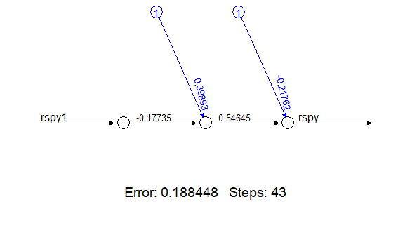
4. References.
[1] C. M. Bishop, “Neural Networks for Pattern Recognition”, Oxford University Press, 1995.
[2] Jeffrey A. Ryan and Joshua M. Ulrich. “quantmod: Quantitative Financial Modelling Framework”. R package version 0.4-15. 2019.
Stefan Fritsch, Frauke Guenther and Marvin N. Wright. “neuralnet: Training of Neural Networks”. R package version 1.44.2. 2019