Last Update: February 14, 2020
Strategy indicators consist of identifying trend-following or mean-reversion asset price patterns. Main indicators include single or multiple, lagging or leading technical indicators.
This topic is part of Advanced Trading Analysis with Python course. Feel free to take a look at Course Curriculum.
This tutorial has an educational and informational purpose and doesn’t constitute any type of trading or investment advice. All content, including code and data, is presented for personal educational use exclusively and with no guarantee of exactness of completeness. Past performance doesn’t guarantee future results. Please read full Disclaimer.
An example of mean-reversion leading strategy indicator is relative strength index RSI [1] which consists of bounded oscillator that measures an asset prices trend strength or weakness. Fourteen days are commonly used for its calculation.
1. Strategy indicator calculation.
1.1. Average gain and loss calculation.
Where = current period close prices fourteen days average gain,
= current period close prices fourteen days average loss absolute value,
= initial close prices fourteen days average gain,
= initial close prices fourteen days average loss absolute value,
= current period close prices gain,
= current period close prices loss absolute value,
= current period close prices gain or loss,
= current period close prices.
1.2. Relative strength calculation.
Where = current period close prices fourteen days relative strength,
= current period close prices fourteen days average gain,
= current period close prices fourteen days average loss absolute value.
1.3. Relative strength index calculation.
Where = current period close prices fourteen days relative strength index,
= current period close prices fourteen days relative strength.
2. Python code example.
2.1. Import Python packages [2].
import numpy as np
import pandas as pd
import matplotlib.pyplot as plt
import talib as ta
2.2. RSI strategy indicator data reading.
- Data: S&P 500® index replicating ETF (ticker symbol: SPY) daily open, high, low, close, adjusted close prices and volume (2016).
SPY = pd.read_csv('Data//RSI-Strategy-Indicator-Data.txt', index_col='Date', parse_dates=True)2.3. RSI strategy indicator calculation and chart.
- Relative strength index RSI strategy indicator number of periods not fixed and only included for educational purposes.
SPY['RSI'] = ta.RSI(np.asarray(SPY['SPY.Close']), timeperiod=14)
fig1, ax = plt.subplots(2, sharex=True)
ax[0].plot(SPY['SPY.Close'])
ax[0].legend(loc='upper left')
ax[1].plot(SPY['RSI'], color='green')
ax[1].legend(loc='upper left')
plt.suptitle('SPY Close Prices & Relative Strength Index RSI(14) Strategy Indicator')
plt.show()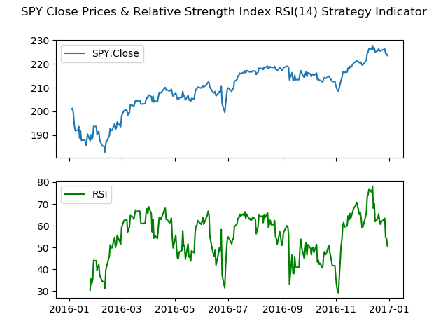
3. References.
[1] J. Welles Wilder Jr. “New Concepts in Technical Trading Systems”. Commodities Magazine (now Futures Magazine). 1978.
[2] Travis E, Oliphant. “A guide to NumPy”. USA: Trelgol Publishing. 2006.
Stéfan van der Walt, S. Chris Colbert and Gaël Varoquaux. “The NumPy Array: A Structure for Efficient Numerical Computation”. Computing in Science & Engineering. 2011.
Wes McKinney. “Data Structures for Statistical Computing in Python.” Proceedings of the 9th Python in Science Conference. 2010.
John D. Hunter. “Matplotlib: A 2D Graphics Environment.” Computing in Science & Engineering. 2007.
Mario Fortier, TicTacTec LLC. “TA-Lib: Technical Analysis Library”. 1999, 2007.
Quantopian. “TA-Lib: Technical Analysis Library”. Python package version 0.4.9. 2018.