Last Update: March 2, 2020
Multiple regression assumptions consist of independent variables correct specification, independent variables no linear dependence, regression correct functional form, residuals no autocorrelation, residuals homoscedasticity and residuals normality.
This topic is part of Multiple Regression Analysis with Python course. Feel free to take a look at Course Curriculum.
This tutorial has an educational and informational purpose and doesn’t constitute any type of business, forecasting, trading or investment advice. All content, including code and data, is presented for personal educational use exclusively and with no guarantee of exactness of completeness. Past performance doesn’t guarantee future results. Please read full Disclaimer.
No linear dependence or no multicollinearity consists of regression independent variables not being highly correlated.
This is evaluated through multicollinearity test which consists of calculating an inverted correlation matrix of independent variables and assessing its main diagonal values.
- If main diagonal values were greater than five but less than ten, independent variables might have been highly correlated.
- If main diagonal values were greater than ten, independent variables were highly correlated.
1. Python code example.
1.1. Import Python packages [1].
import numpy as np
import pandas as pd
import matplotlib.pyplot as plt
1.2. Multicollinearity test data.
- Data: S&P 500® index replicating ETF (ticker symbol: SPY) adjusted close prices arithmetic monthly returns, 1 Year U.S. Treasury Bill Yield, 10 Years U.S. Treasury Note Yield, Merrill Lynch U.S. High Yield Corporate Bond Index Yield effective monthly yields, U.S. Consumer Price Index, U.S. Producer Price Index monthly inflations or deflations, West Texas Intermediate Oil prices arithmetic monthly returns, U.S. Industrial Production Index value, U.S. Personal Consumption Expenditures arithmetic monthly changes (1997-2016).
data = pd.read_csv('Data//Multicollinearity-Test-Data.txt', index_col='Date', parse_dates=True)1. 3. Multicollinearity test calculation and chart.
- Multicollinearity test done only on independent variables.
ivar = data[['t1y', 't10y', 'hyield', 'cpi', 'ppi', 'oil', 'indpro', 'pce']]In:
pd.set_option('display.max_columns', 8)
print('== Inverted Correlation Matrix ==')
print('')
print(pd.DataFrame(np.linalg.inv(ivar.corr()), index=ivar.columns, columns=ivar.columns))Out:
t1y t10y hyield cpi ppi oil indpro \
t1y 5.467935 -5.272915 0.776502 -0.275036 0.570422 -0.024870 0.356823
t10y -5.272915 6.617777 -1.630708 -0.016011 -0.584221 0.133328 -0.792149
hyield 0.776502 -1.630708 1.797855 0.156680 0.300730 -0.160866 0.649356
cpi -0.275036 -0.016011 0.156680 2.708274 -1.848520 -0.144473 0.265487
ppi 0.570422 -0.584221 0.300730 -1.848520 3.079372 -0.922318 -0.112324
oil -0.024870 0.133328 -0.160866 -0.144473 -0.922318 1.686173 -0.033936
indpro 0.356823 -0.792149 0.649356 0.265487 -0.112324 -0.033936 1.353335
pce -0.023391 -0.277448 0.285020 -0.396875 0.082269 -0.184198 -0.195657
pce
t1y -0.023391
t10y -0.277448
hyield 0.285020
cpi -0.396875
ppi 0.082269
oil -0.184198
indpro -0.195657
pce 1.365534fig = plt.figure()
ax = fig.add_subplot(111)
cax = ax.matshow(np.linalg.inv(ivar.corr()), cmap='Blues')
fig.colorbar(cax)
ax.set_xticklabels([''] + ['t1y', 't10y', 'hyield', 'cpi', 'ppi', 'oil', 'indpro', 'pce'])
ax.set_yticklabels([''] + ['t1y', 't10y', 'hyield', 'cpi', 'ppi', 'oil', 'indpro', 'pce'])
ax.set_title('Inverted Correlation Matrix')
plt.show()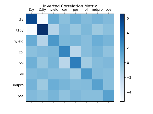
2. References.
[1] Travis E, Oliphant. “A guide to NumPy”. USA: Trelgol Publishing. 2006.
Stéfan van der Walt, S. Chris Colbert and Gaël Varoquaux. “The NumPy Array: A Structure for Efficient Numerical Computation”. Computing in Science & Engineering. 2011.
Wes McKinney. “Data Structures for Statistical Computing in Python.” Proceedings of the 9th Python in Science Conference. 2010.
John D. Hunter. “Matplotlib: A 2D Graphics Environment.” Computing in Science & Engineering. 2007.