MACD Stock Technical Indicator with Python

Last Update: February 6, 2020

Stock technical indicators are calculated by applying certain formula to stock prices and volume data. They are used to alert on the need to study stock price action with greater detail, confirm other technical indicators’ signals or predict future stock prices direction.

This topic is part of Stock Technical Analysis with Python course. Feel free to take a look at Course Curriculum.

This tutorial has an educational and informational purpose and doesn’t constitute any type of trading or investment advice. All content, including code and data, is presented for personal educational use exclusively and with no guarantee of exactness of completeness. Past performance doesn’t guarantee future results. Please read full Disclaimer.

An example of stock technical indicators is moving averages convergence/divergence MACD [1] which consists of centered oscillator that measures a stock price momentum and identifies trends. Twelve days are commonly used for short-term smoothing, twenty-six days for long-term smoothing and nine days for signal.

1. Technical indicator calculation.

1.1. Short-term and long-term smoothing calculation.

Where = current period stock close prices, = current period close prices periods exponential moving average, = initial close prices periods simple moving average.

1.2. Moving averages convergence/divergence MACD stock technical indicator, signal and histogram calculation.

Where = current period close prices MACD, = current period close prices MACD signal,  = current period close prices MACD histogram.

2. Python code example.

2.1. Import Python packages [2].

import numpy as np
import pandas as pd
import matplotlib.pyplot as plt
import talib as ta

2.2. MACD stock technical indicator data reading.

• Data: S&P 500® index replicating ETF (ticker symbol: SPY) daily open, high, low, close, adjusted close prices and volume (2016).

SPY = pd.read_csv('Data//MACD-Stock-Technical-Indicator-Data.txt', index_col='Date', parse_dates=True)

2.3. MACD stock technical indicator calculation and chart.

• MACD technical indicator, signal and histogram number of periods not fixed and only included for educational purposes.

SPY['macd'], SPY['macdsig'], SPY['macdhist'] = ta.MACD(np.asarray(SPY['SPY.Close']),
                                                      fastperiod=12, slowperiod=26, signalperiod=9)

fig1, ax = plt.subplots(2, sharex=True)
ax[0].plot(SPY['SPY.Close'])
ax[0].legend(loc='upper left')
ax[1].plot(SPY['macd'])
ax[1].plot(SPY['macdsig'])
ax[1].plot(SPY['macdhist'], linestyle='--')
ax[1].legend(loc='upper left')
plt.suptitle('SPY Close Prices and MACD(12,26,9) Stock Technical Indicator')
plt.show()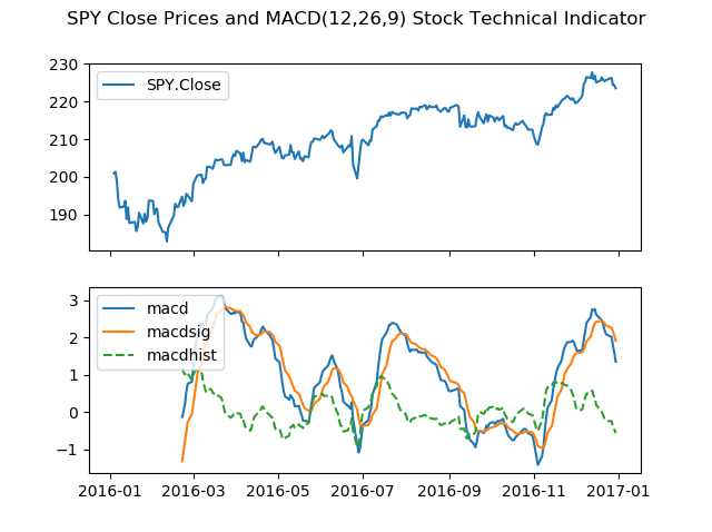

3. References

[1] Gerald Appel. “Technical Analysis: Powerful Tools for Active Investors”. FT Press. 2005.

[2] Travis E, Oliphant. “A guide to NumPy”. USA: Trelgol Publishing. 2006.

Stéfan van der Walt, S. Chris Colbert and Gaël Varoquaux. “The NumPy Array: A Structure for Efficient Numerical Computation”. Computing in Science & Engineering. 2011.

Wes McKinney. “Data Structures for Statistical Computing in Python.” Proceedings of the 9th Python in Science Conference. 2010.

John D. Hunter. “Matplotlib: A 2D Graphics Environment.” Computing in Science & Engineering. 2007.

Mario Fortier, TicTacTec. “TA-Lib: Technical Analysis Library”. 1999, 2007.

Quantopian. “TA-Lib: Technical Analysis Library”. Python package version 0.4.9. 2018.