Last Update: February 6, 2020
Exponential smoothing methods consist of forecast based on previous periods data with exponentially decaying influence the older they become. Their notation is ETS (error, trend, seasonality) where each can be none (N), additive (A), additive damped (Ad), multiplicative (M) or multiplicative damped (Md).
This topic is part of Forecasting Models with Python course. Feel free to take a look at Course Curriculum.
This tutorial has an educational and informational purpose and doesn’t constitute any type of forecasting, business, trading or investment advice. All content, including code and data, is presented for personal educational use exclusively and with no guarantee of exactness of completeness. Past performance doesn’t guarantee future results. Please read full Disclaimer.
An example of exponential smoothing methods is Brown simple exponential smoothing [1] which consists of forecast with no trend or seasonal patterns.
1. Method notation.
• ETS(A,N,N): error = additive, trend = none, seasonality = none
2. Formula notation.
Where =
step forecast,
= current period level forecast,
= current period data,
= level smoothing coefficient.
3. Python code example.
3.1. Import Python packages [2].
import pandas as pd
import matplotlib.pyplot as plt
import statsmodels.tsa.holtwinters as ets
3.2. Exponential smoothing methods data reading, training and testing ranges delimiting.
- Data: S&P 500® index replicating ETF (ticker symbol: SPY) daily adjusted close prices (2007-2015).
- Training and testing ranges delimiting not fixed and only included for educational purposes.
spy = pd.read_csv('Data//Exponential-Smoothing-Methods-Data.txt', index_col='Date', parse_dates=True)
spy = spy.asfreq('B')
spy = spy.fillna(method='ffill')

spyt = spy[:'2013-12-31']
spyf = spy['2014-01-02':]
3.3. Brown simple exponential smoothing method calculation and chart.
brownt = ets.ExponentialSmoothing(spyt, trend=None, damped=False, seasonal=None).fit()
brownf = brownt.forecast(steps=len(spyf))

fig1, ax = plt.subplots()
ax.plot(spyt, label='spyt')
ax.plot(spyf, label='spyf')
ax.plot(brownf, label='brownf')
plt.legend(loc='upper left')
plt.title('Brown Simple Exponential Smoothing ETS(A,N,N) Method')
plt.ylabel('Price')
plt.xlabel('Date')
plt.show()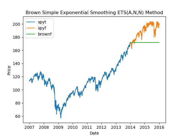
References.
[1] Robert G. Brown. “Exponential Smoothing for Predicting Demand”. Arthur D. Little Inc. 1956.
[2] Wes McKinney. “Data Structures for Statistical Computing in Python.” Proceedings of the 9th Python in Science Conference. 2010.
John D. Hunter. “Matplotlib: A 2D Graphics Environment.” Computing in Science & Engineering. 2007.
Seabold, Skipper, and Josef Perktold. “Statsmodels: Econometric and statistical modeling with python.” Proceedings of the 9th Python in Science Conference. 2010.