Last Update: December 22, 2020
First order trend stationary time series consist of random processes that have constant mean which don’t exhibit trend pattern.
This topic is part of Pairs Trading Analysis with Python course. Feel free to take a look at Course Curriculum.
This tutorial has an educational and informational purpose and doesn’t constitute any type of trading or investment advice. All content, including code and data, is presented for personal educational use exclusively and with no guarantee of exactness of completeness. Past performance doesn’t guarantee future results. Please read full Disclaimer.
Augmented Dickey-Fuller test [1] consists of evaluating whether time series was first order trend stationary with null hypothesis that it had a unit root and was not stationary.
1. Formula notation.
1.1. Augmented Dickey-Fuller test formula notation.
Where = current period asset prices difference,
= regression constant term,
= regression coefficients,
= linear trend variable,
= previous period asset price,
= previous periods asset prices differences,
= number of lags included within test,
= regression residuals or forecasting errors.
1.2. Augmented Dickey-Fuller test formula notation constant and linear trend variable assumptions options.
Where = regression constant term,
= linear trend variable regression coefficient.
1.3. Augmented Dickey-Fuller test.
Augmented Dickey-Fuller individual test coefficient t-statistic approximated
:
- If Augmented Dickey-Fuller individual test
coefficient t-statistic approximated
level of statistical significance then time series was first order trend stationary with
level of statistical confidence.
- If Augmented Dickey-Fuller individual test
level of statistical significance then higher differentiation order needed for first order trend stationary time series with
2. Python code example.
2.1. Import Python packages [2].
import numpy as np
import pandas as pd
import matplotlib.pyplot as plt
import statsmodels.tsa.stattools as ts
2.2. Augmented Dickey-Fuller test data reading, training and testing ranges delimiting.
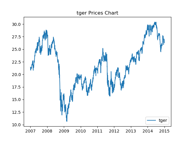
- Data: MSCI® Germany index replicating ETF (ticker symbol: EWG) daily adjusted close prices (2007-2016).
- Training and testing ranges delimiting not fixed and only included for educational purposes.
data = pd.read_csv('Data//Augmented-Dickey-Fuller-Test-Data.txt', index_col='Date', parse_dates=True)tdata = data[:'2014-12-31']
tdata.columns = ['tger']
fdata = data['2015-01-02':]
fdata.columns = ['fger']
2.3. Augmented Dickey-Fuller test prices chart.
- Augmented Dickey-Fuller test prices chart within training range.
tger = tdata
fig1, ax = plt.subplots()
ax.plot(tger, label='tger')
ax.legend(loc='lower right')
plt.title('tger Prices Chart')
plt.show()
2.4. Augmented Dickey-Fuller test calculation and output.
- Augmented Dickey-Fuller test calculation within training range.
- Augmented Dickey-Fuller test function maximum lag order, constant and linear trend assumptions not fixed and only included for educational purposes.
tgeradf = ts.adfuller(tger, maxlag=1, regression='ct')In:
print('== Prices Augmented Dickey-Fuller Test ==')
print('')
print('Augmented Dickey-Fuller ADF Test Statistic: ', np.round(tgeradf[0], 6))
print('Augmented Dickey-Fuller ADF Test P-Value: ', np.round(tgeradf[1], 6))
Out:
== Prices Augmented Dickey-Fuller Test ==

Augmented Dickey-Fuller ADF Test Statistic:  -1.784965
Augmented Dickey-Fuller ADF Test P-Value:  0.711963
3. References.
[1] David A. Dickey and Wayne A. Fuller. “Distribution of the Estimators for Autoregressive Time Series with a Unit Root”. Journal of the American Statistical Association. 1979.
[2] Travis E, Oliphant. “A guide to NumPy”. USA: Trelgol Publishing. 2006.
Stéfan van der Walt, S. Chris Colbert and Gaël Varoquaux. “The NumPy Array: A Structure for Efficient Numerical Computation”. Computing in Science & Engineering. 2011.
Wes McKinney. “Data Structures for Statistical Computing in Python.” Proceedings of the 9th Python in Science Conference. 2010.
John D. Hunter. “Matplotlib: A 2D Graphics Environment.” Computing in Science & Engineering. 2007.
Seabold, Skipper, and Josef Perktold. “Statsmodels: Econometric and statistical modeling with python.” Proceedings of the 9th Python in Science Conference. 2010.