Last Update: February 6, 2020
Exponential smoothing methods consist of forecast based on previous periods data with exponentially decaying influence the older they become. Their notation is ETS (error, trend, seasonality) where each can be none (N), additive (A), additive damped (Ad), multiplicative (M) or multiplicative damped (Md).
This topic is part of Forecasting Models with Excel course. Feel free to take a look at Course Curriculum.
This tutorial has an educational and informational purpose and doesn’t constitute any type of forecasting, business, trading or investment advice. All content, including spreadsheet calculations and data, is presented for personal educational use exclusively and with no guarantee of exactness of completeness. Past performance doesn’t guarantee future results. Please read full Disclaimer.
An example of exponential smoothing methods is Brown simple exponential smoothing [1] which consists of forecast with no trend or seasonal patterns.
1. Method notation.
- ETS(A,N,N): error = additive, trend = none, seasonality = none
2. Formula notation.
Where =
step forecast,
= current period level forecast,
= current period data,
= level smoothing coefficient.
3. Excel example.
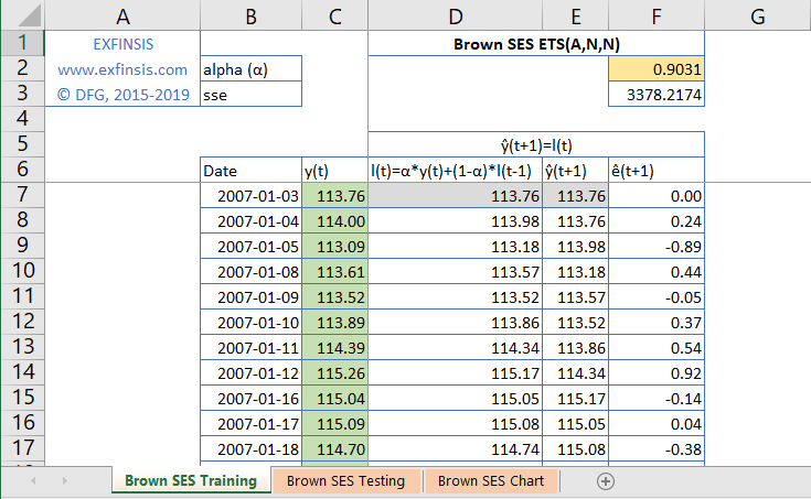
3.1. Exponential smoothing methods level smoothing coefficient estimation within training range.
- Data: S&P 500® index replicating ETF (ticker symbol: SPY) daily adjusted close prices (2007-2013).
- Training range delimiting not fixed and only included for educational purposes.
- Level smoothing coefficient estimation done through sum of squared errors (sse) constrained minimization using Microsoft Excel Solver® Add-In.
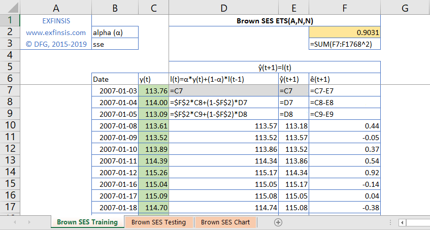
3.2. Exponential smoothing methods level smoothing coefficient estimation formulas within training range.
- Initial forecasts assumptions not fixed and only included for educational purposes.
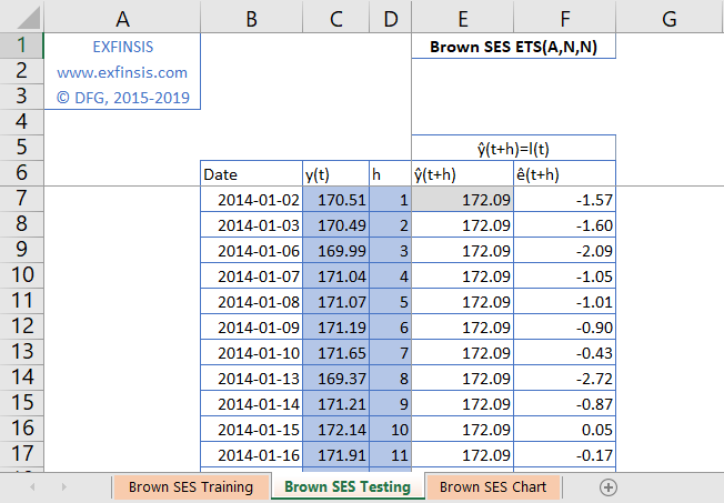
3.3. Exponential smoothing methods multi-steps forecast within testing range.
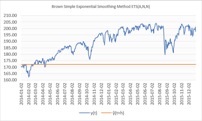
- Data: S&P 500® index replicating ETF (ticker symbol: SPY) daily adjusted close prices (2014-2015).
- Testing range delimiting not fixed and only included for educational purposes.
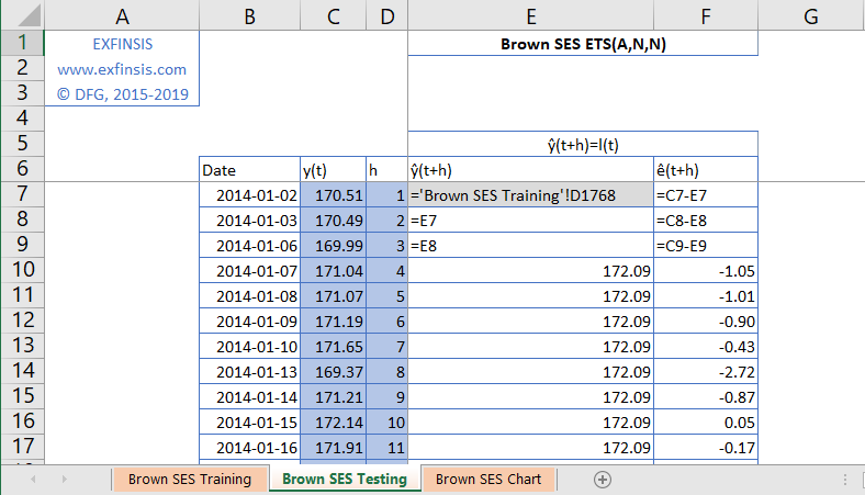
3.4. Exponential smoothing methods multi-steps forecast formulas within testing range.
3.5. Exponential smoothing methods multi-steps forecast chart within testing range.
References.
[1] Robert G. Brown. “Exponential Smoothing for Predicting Demand”. Arthur D. Little Inc. 1956.