Last Update: February 12, 2020
Asset pricing models consist of estimating asset expected return through its expected risk premium linear relationship with factors portfolios expected risk premiums and macroeconomic factors.
This topic is part of Investment Portfolio Analysis with Excel course. Feel free to take a look at Course Curriculum.
This tutorial has an educational and informational purpose and doesn’t constitute any type of trading or investment advice. All content, including spreadsheet calculations and data, is presented for personal educational use exclusively and with no guarantee of exactness of completeness. Past performance doesn’t guarantee future results. Please read full Disclaimer.
An example of asset pricing models is capital asset pricing model CAPM [1] which consists of estimating asset expected return through its expected risk premium linear relationship with market expected risk premium.
- CAPM Beta coefficient consists of estimating asset market systematic risk through the linear relationship between asset and market risk premiums.
- Jensen’s alpha [2] consists of estimating asset average realized excess return through the difference between asset average realized return and its estimated expected return using capital asset pricing model CAPM.
1. Formula notation.
1.1. Capital asset pricing model CAPM formula notation.
Where = asset expected return,
= expected risk free return,
= asset CAPM beta coefficient,
= market expected risk premium.
1.2. CAPM Beta coefficient formula notation.
Where = risk free return,
= constant,
= asset CAPM beta coefficient,
= asset and market returns covariance,
= market returns variance,
= asset and market risk premiums covariance,
= market risk premiums variance.
1.3. Jensen’s alpha formula notation.
- Note: CAPM formula recasting using average realized returns (ex-post) instead of expected returns (ex-ante). For full reference, please read Jensen’s alpha [2].
Where = asset average realized excess return,
= asset average realized return,
= average realized risk free return,
= asset CAPM beta coefficient,
= market average realized return.
2. Excel example.
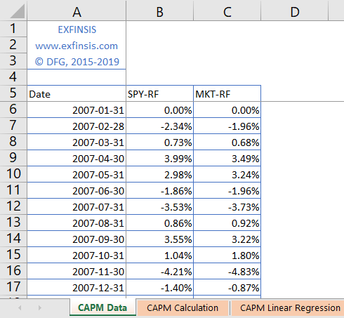
2.1. CAPM single factor model data.
- Data: S&P 500® index replicating ETF (ticker symbol: SPY) adjusted close prices and market portfolio [3] monthly arithmetic returns risk premiums (2007-2016).
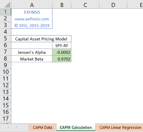
2.2. CAPM Single Factor Model Calculation.
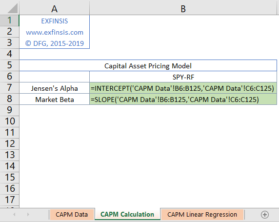
2.3. CAPM Single Factor Model Calculation Formulas.
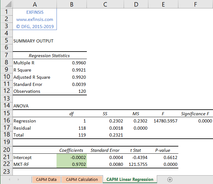
2.4. CAPM Single Factor Model Linear Regression Calculation.
- Linear regression calculation done using Microsoft Excel Data Analysis® Add-In Regression Analysis Tool.
3. References
[1] Jack Treynor (1961, 1962), William F. Sharpe (1964), John Lintner (1965), Jan Mossin (1966). Craig W. French. “The Treynor Capital Asset Pricing Model”. Journal of Investment Management. 2003.
[2] Michael C. Jensen. “The Performance of Mutual Funds in the Period 1945-1964”. Journal of Finance. 1968.
[3] Eugene F. Fama and Kenneth F. French. “Common Risk Factors in the Returns on Stocks and Bonds,” Journal of Financial Economics. 1993.